SVM Algorithm Explained: A Complete Practical Guide

In machine learning, many datasets cannot be separated using a simple decision boundary. This is where Support Vector Machine (SVM) proves its strength. From image classification to spam detection and text analysis, SVM remains one of the most widely used algorithms for classification tasks. This article explores how SVM works, why it is effective, and where it is used in various applications.

In this article:

1. What is a Support Vector Machine?

2. A Brief History — Soviet Roots to Silicon Valley

3. How SVM Works — The Intuition

4. The Mathematics Behind SVM

5. The Kernel Trick — SVM's Secret Weapon

6. Types of SVM

7. The SVM Workflow — Step by Step

8. Implementing SVM in Python (scikit-learn)

9. Real-World Applications

10. 2024–2025 Benchmarks and Research Findings

11. Strengths and Limitations

12. Why SVM Still Matters in 2025 — Deep Learning Era

13. Where SVM Fails — Failure Analysis & Production Gaps

14. Hybrid CNN-SVM, Explainable AI (SHAP/LIME), and Quantum SVM

15. SVM vs. Other Algorithms

16. Expert Tips for Getting the Best from SVM

17. Key Takeaways

    

What Is a Support Vector Machine (SVM)?

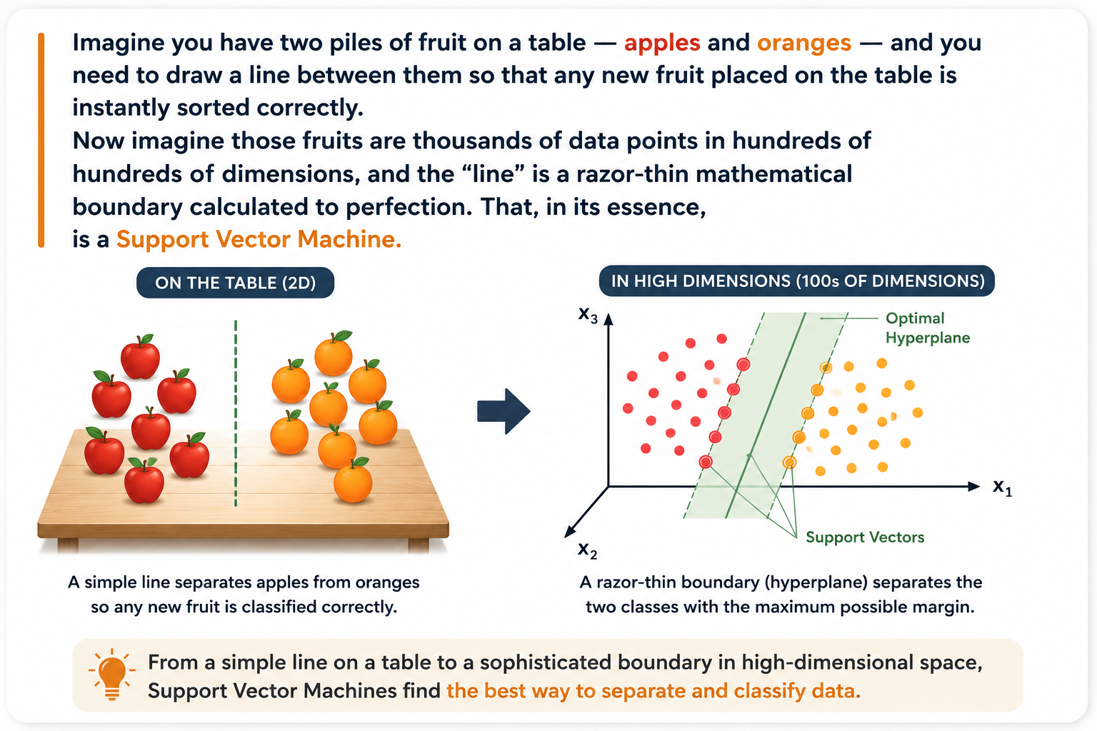
A Support Vector Machine (SVM) is a supervised machine learning algorithm. It is designed to find the best possible boundary — referred to as a hyperplane — that separates data into two or more classes. The algorithm serves as one of the most theoretically established methods which effectively enables ML practitioners to classify data sets. SVM serves multiple fields through its ability to solve both classification and regression tasks which extend to applications in signal processing, natural language processing, and image recognition.

SVM is special not because of its ability to separate data; this is done by many other algortihms. The special feature of SVM operates through its system which helps in maximization of the margin between its hyperplane and the nearest boundary points in both directions. This maximum-margin philosophy is the source of its power, elegance, and robustness.

Core Definition

SVM is a supervised learning algorithm that works by finding an optimal decision boundary (hyperplane) that maximizes the margin between two classes. The data points lying closest to this boundary are called support vectors — they are the only data points that actually define where the boundary sits.

A Brief History — Soviet Roots to Silicon Valley

The story of SVM is one of the most fascinating in all of computer science — spanning Cold War mathematics, Bell Labs innovation, and a global machine learning revolution.

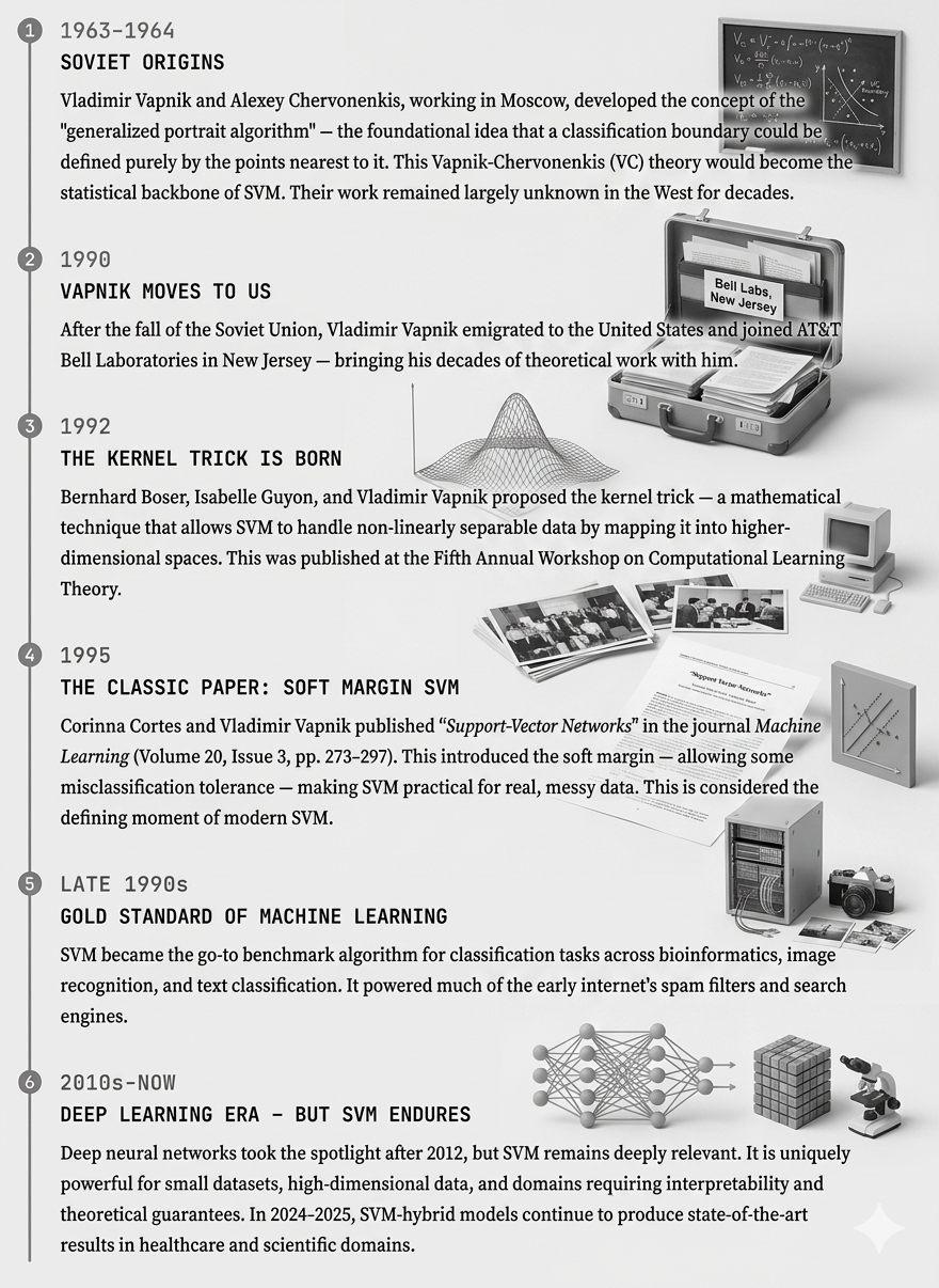
"SVMs are one of the most robust prediction methods, based on the statistical learning framework of VC theory."

— Vladimir Vapnik, co-inventor of SVM; cited in NCBI Bookshelf, Springer Nature (2022)

How SVM Works — The Intuition, Explained Simply

Before diving into the mathematical foundations, it is important to establish a strong conceptual understanding.

Step 1: The Problem — Drawing a Line Between Two Groups

Let’s suppose you have data points on a 2D plane — some are red dots and some are blue dots. You want a boundary such that whenever there’s a new point coming in, it will fall into the right class. There are infinitely many possible lines you could draw. Which one is the best?

Step 2: The SVM Answer — Maximize the Gap

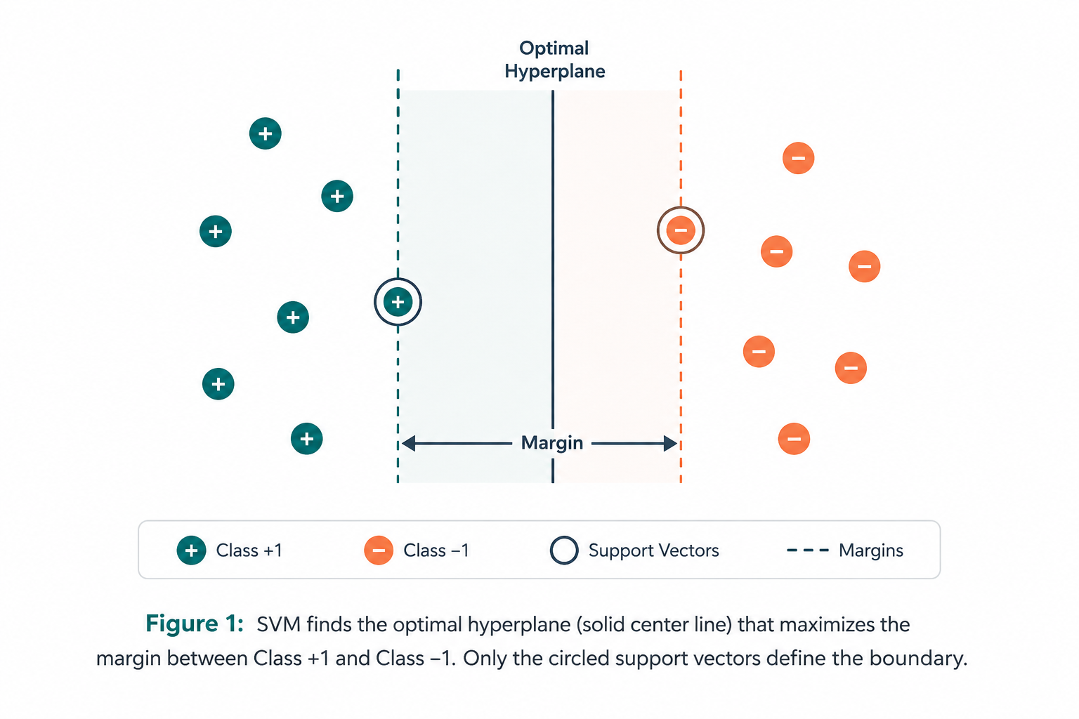
SVM's answer is: choose the line that is as far as possible from both groups simultaneously. This maximum-gap line is called the optimal hyperplane. The empty space on either side of the hyperplane — the "safety zone" — is called the margin.

Why Bigger Margin = Better Model

A wider margin means the model has more "breathing room." It is less likely to misclassify new data that falls slightly differently from the training data. This is the heart of SVM's excellent generalization performance.

Step 3: Support Vectors — The VIPs of the Dataset

Among all your data points, only a small subset actually matters for drawing the boundary — the points that sit right at the edge of each class, closest to the decision line. These elite data points are the support vectors. Remove any other point from your dataset and the boundary stays exactly the same. Remove a support vector, and everything shifts.

As defined by MathWorks, "The data points that mark the boundary of this parallel slab and are closest to the separating hyperplane are the support vectors. Support vectors refer to a subset of the training observations that identify the location of the separating hyperplane."

Step 4: What If Data Can't Be Separated by a Straight Line?

Real-world data is rarely neatly split into two tidy groups. Sometimes red and blue dots are mixed together in complex patterns. This is where SVM gets truly clever — through something called the kernel trick, it mathematically lifts the data into a higher-dimensional space where a clean boundary suddenly becomes possible. We'll explore this fully in the coming sections.

Read Also: Top 25 Data Science Companies in India - Career in Data Science

The Mathematics Behind SVM

You don't need a PhD to understand SVM's math — just a calm, step-by-step walk through the key ideas. Let's do exactly that.

The Hyperplane Equation

In two dimensions, a hyperplane is simply a line. In three dimensions, it's a flat plane. In n dimensions, it's an n−1 dimensional surface. Mathematically, SVM's decision boundary is described as:

The Hyperplane Equation

wTx + b = 0

Where w is the weight vector (perpendicular to the hyperplane, pointing in the direction of classification), x is the input feature vector, and b is the bias term (controlling how far the hyperplane is from the origin)

Classifying a New Point

Given a new data point x, SVM classifies it based on which side of the hyperplane it falls on:

Classification Rule

ŷ = +1 if wTx + b ≥ 0  |  ŷ = −1 if wTx + b < 0

The Margin and What We're Optimizing

The geometric margin is the perpendicular distance from the hyperplane to the nearest data point. The total margin width is 2 / ‖w‖. To maximize this margin, we minimize ‖w‖², which leads to SVM's classic optimization problem:

Hard-Margin Optimization (Linearly Separable Data)

Minimize: ½ ‖w‖²

Subject to: yi(wTxi + b) ≥ 1   for all i

This is a quadratic programming (QP) problem — it has a unique global solution, which means SVM always converges to the same optimal boundary, unlike neural networks which can get stuck in local minima.

Soft Margin — Handling Real, Messy Data

Real data is never perfectly separable. The soft margin SVM (introduced by Cortes and Vapnik, 1995) introduces slack variables ξi that allow some data points to violate the margin or even be misclassified. The cost is controlled by the hyperparameter C:

Soft-Margin Optimization (Non-Separable Data)

Minimize: ½ ‖w‖² + C · Σ ξi

Subject to: yi(wTxi + b) ≥ 1 − ξi   and   ξi ≥ 0

Understanding the C Hyperparameter

• High C: Small tolerance for errors → narrow margin → risk of overfitting (memorizing training data).

• Low C: More tolerance for errors → wide margin → risk of underfitting. The right C balances generalization and accuracy.

The Hinge Loss Function

SVMs punish wrong predictions i.e. misclassified or margin-violating points using something called hinge loss. Here is how it works: A point gets zero penalty when it lands in the right place with enough margin. But if it falls too close (inside the margin) or on the wrong side, the penalty goes up with the distance of the mistake.

Hinge Loss

L = max(0, 1 − yi · (wTxi + b))

The Dual Problem — Unlocking the Kernel Trick

With the application of Lagrange multipliers, SVM's optimization problem can be rewritten in a form known as the dual problem. This reformulation is critical because it allows SVM to work with kernel functions. In the dual form, all computations involve dot products of data points — and dot products can be replaced by kernel functions to implicitly handle higher dimensions without ever computing the actual coordinates there.

Dual Objective Function

Maximize: Σ αi − ½ · Σi,j αi αj yi yj K(xi, xj)

Subject to: 0 ≤ αi ≤ C   and   Σ αi yi = 0

Where αi are Lagrange multipliers and K(xi, xj) is the kernel function. The support vectors are exactly the training points where αi > 0.

Kernel Trick — SVM's Secret Weapon

This is arguably the most important concept in all of SVM theory. Understanding it will transform how you think about machine learning.

Problem: What If Data Isn't Linearly Separable?

Imagine dots arranged in concentric circles — inner circle is one class, outer circle is another. No straight line can separate them. What do you do?

Solution: Project to Higher Dimensions

The idea: add a new dimension. For example, if your 2D points are (x1, x2), create a third dimension z = x1² + x2². The concentric circles, when viewed in 3D from above, separate into different height layers that can now be cut by a flat plane. A hyperplane in 3D becomes a curved boundary when projected back to 2D.

The catch: Computing coordinates in very high or infinite dimensions is computationally explosive. This is where the kernel trick saves the day.

The Kernel Trick Explained

A kernel function K(xi, xj) computes the dot product of two points in the higher-dimensional space without ever explicitly computing their coordinates in that space. This means SVM can work in infinite-dimensional spaces at the computational cost of a simple function evaluation. It is both mathematically elegant and computationally miraculous.

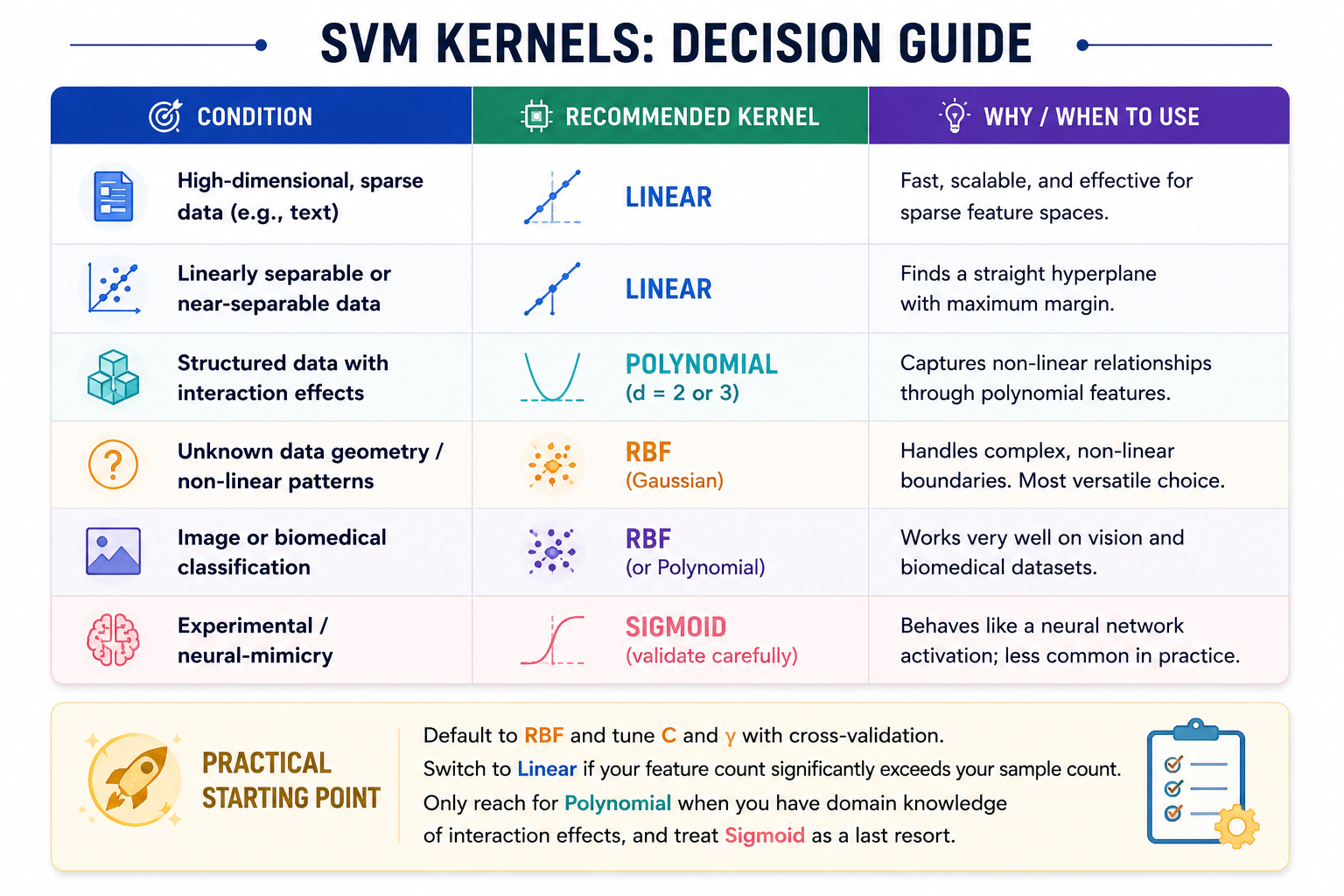
Rule of Thumb: Which Kernel to Pick?

Start with RBF (Radial Basis Function). It is the default in scikit-learn and performs well in most situations. Use Linear when you have many features relative to training samples (e.g., text data). Try Polynomial when you suspect polynomial relationships in your features.

"The kernel trick is one of the most elegant ideas in all of machine learning — it allows computation in infinite-dimensional spaces at finite cost."

— Bernhard Schölkopf, Director, Max Planck Institute for Intelligent Systems; widely cited in kernel methods literature

Types of SVM

1. Linear SVM (Hard Margin)

Used when data is perfectly linearly separable. Draws a single straight line (in 2D), plane (in 3D), or hyperplane (in n-D) with zero tolerance for misclassification. Rarely applicable to real-world data but conceptually foundational.

2. Soft Margin SVM

The practical version of SVM for real, imperfect data. Allows some data points to be on the wrong side of the margin, controlled by the hyperparameter C. This is the default SVC in scikit-learn.

3. Non-Linear SVM (Kernel SVM)

Uses a kernel function to project data into a higher-dimensional space where it becomes linearly separable. The most powerful and commonly used variant. Applications include image recognition, bioinformatics, and medical diagnostics.

4. Support Vector Regression (SVR)

SVM adapted for continuous numerical prediction rather than classification. Instead of maximizing the margin between classes, SVR fits a function within an epsilon-tube around the data, tolerating small errors while penalizing larger ones. Extremely useful for financial forecasting and time-series prediction.

5. One-Class SVM

A variant for anomaly detection. Trained on normal data only, it learns a boundary around "normal" — anything outside that boundary is flagged as an anomaly. Used in fraud detection, network intrusion detection, and manufacturing quality control.

6. Multi-Class SVM

SVM is natively binary, but multi-class problems are solved using:

• One-vs-One (OvO): Trains a classifier for every pair of classes; the most popular class wins by vote.

• One-vs-Rest (OvR): Trains one classifier per class (this class vs. all others); the most confident classifier's class wins.

SVM Workflow — Step by Step

1. Data Collection & Preprocessing

Gather labeled training data. Handle missing values, remove outliers, and encode categorical variables. SVM is sensitive to feature scale — always normalize or standardize your features (zero mean, unit variance) using StandardScaler. Without this, features with larger numeric ranges will dominate the margin calculation.

2. Feature Engineering & Dimensionality Reduction

SVM performs best with informative, non-redundant features. Consider PCA to reduce dimensions while preserving variance. A 2024 study published in Nature Scientific Reports showed that adding PCA before SVM improved brain tumor MRI classification accuracy from 86.57% to 94.20%.

3. Train-Test Split with Cross-Validation

Split your data into training (typically 70–80%) and test (20–30%) sets. Use k-fold cross-validation during model selection to get reliable performance estimates and avoid overfitting to a single split.

4. Choose the Right Kernel

Select your kernel based on data characteristics. When in doubt, start with RBF. For very high-dimensional sparse text data, linear kernel is often faster and equally effective.

5. Train the SVM Model

Fit the SVM to your training data. Under the hood, this solves the quadratic programming optimization problem to find the support vectors and the optimal hyperplane. The solver used in scikit-learn (libsvm) is highly optimized.

6. Hyperparameter Tuning

Tune C (regularization), gamma (RBF kernel width), and degree (for polynomial kernel) using Grid Search or Bayesian Optimization with cross-validation. This step can dramatically improve performance — the difference between a mediocre and excellent SVM model often lies here.

7. Evaluation & Interpretation

Measure accuracy, precision, recall, F1-score, and ROC-AUC on the test set. For imbalanced datasets, accuracy alone can be misleading — always examine the confusion matrix and class-wise metrics.

Kernel Types & When to Use Them

The kernel function is the mathematical core of an SVM. It quietly maps your data into a higher-dimensional space. There, a straight line can separate classes that looked impossible to split before. Picking the right kernel isn't about taste. It's about understanding the shape of your data.

1. Linear Kernel

Formula: K(x, xᵢ) = xᵀxᵢ

This one just computes a dot product between two vectors. No transformation. No tricks. Just a flat, straight decision boundary.

Use it when you have lots of features but not many training samples. Also use it when your data is already close to linearly separable. In those cases, adding complexity doesn't help. It only slows things down. The linear kernel trains faster than any other option. That matters when you're working at scale.

Key hyperparameter: C — controls how much you penalize misclassifications.

Best for: Text classification, document categorization, TF-IDF features, and any sparse high-dimensional data where linear separation already works well.

Avoid when: Your data has clear curves, feature interactions, or lives in a low-dimensional space.

2. Polynomial Kernel

Formula: K(x, xᵢ) = (γ · xᵀxᵢ + r)^d

This kernel raises the dot product to a power d. It expands the feature space to include polynomial combinations of your original features. That lets the model learn curved boundaries. It's mathematically the same as applying polynomial feature transforms before a linear SVM. But the kernel trick makes it much cheaper to compute.

Key hyperparameters: d — higher degree means more curve but more overfitting risk. r — balances the influence of high vs. low degree terms. γ — scales the dot product.

Best for: Image recognition, genomics, NLP tasks with n-gram interactions, and structured data where feature combinations carry real meaning.

Avoid when: Data is noisy or high-dimensional. Degree tuning gets expensive fast. The kernel is also sensitive to feature scaling, so watch out.

3. RBF (Radial Basis Function) / Gaussian Kernel

Formula: K(x, xᵢ) = exp(−γ‖x − xᵢ‖²)

This kernel measures squared Euclidean distance between two points. The further apart they are, the closer the kernel value gets to zero. Each training point has a localized, bell-shaped influence on the boundary. γ controls how wide or narrow that influence is. High γ means tight local regions — easy to overfit. Low γ means a smoother, more global boundary — easier to underfit.

RBF is the default pick when you know nothing about your data. It handles complex relationships well. In benchmarks, it consistently ranks highest among kernel variants for capturing non-linear patterns.

Key hyperparameters: C and γ — tune both together. Grid search with cross-validation works well. A solid starting point is C ∈ {0.1, 1, 10, 100} and γ ∈ {0.001, 0.01, 0.1, 1}.

Best for: General non-linear classification, images, biomedical signals, and problems where the class geometry is messy or unknown.

Avoid when: Data with very high dimensions and sparsity; text data in its bag-of-words format. Distance metrics become unreliable there. A linear kernel will beat it in those cases.

4. Sigmoid Kernel

Formula: K(x, xᵢ) = tanh(γ · xᵀxᵢ + r)

Sigmoid kernel applies a hyperbolic tangent to the dot product. It mimics what a single-layer neural network does. It's also called the multilayer perceptron kernel for that reason.

It's rarely the right choice though. The decision regions can become non-convex. That breaks the convexity guarantee that makes SVMs reliable. This kernel also fails Mercer's condition for many parameter values, which means that it can behave unpredictably depending on γ and r.

Best for: Experiments where you want neural network-like behavior without building a full network. It is useful in signal processing or bioinformatics occasionally.

Avoid as a default: Without very careful tuning, it offers no real advantage over RBF. It just adds instability for no clear gain.

Implementing SVM in Python — Complete Practical Guide

The most popular SVM implementation is in scikit-learn — considered to be the gold standard Python library for machine learning. This library uses libsvm and liblinear, well-optimized libraries written in C++. The following are some working examples.

Basic Classification with SVM

# Step 1: Import required libraries

from sklearn import datasets

from sklearn.svm import SVC

from sklearn.model_selection import train_test_split

from sklearn.preprocessing import StandardScaler

from sklearn.metrics import classification_report, accuracy_score

# Step 2: Load data (using Iris dataset as example)

iris = datasets.load_iris()

X, y = iris.data, iris.target

# Step 3: Split into train and test sets

X_train, X_test, y_train, y_test = train_test_split(

    X, y, test_size=0.2, random_state=42, stratify=y

)

# Step 4: Scale features — CRITICAL for SVM

scaler = StandardScaler()

X_train = scaler.fit_transform(X_train)

X_test = scaler.transform(X_test)

# Step 5: Train the SVM (RBF kernel by default)

svm_model = SVC(kernel='rbf', C=1.0, gamma='scale', random_state=42)

svm_model.fit(X_train, y_train)

# Step 6: Evaluate

y_pred = svm_model.predict(X_test)

print(f"Accuracy: {accuracy_score(y_test, y_pred):.4f}")

print(classification_report(y_test, y_pred, target_names=iris.target_names))

Hyperparameter Tuning with GridSearchCV

from sklearn.model_selection import GridSearchCV

# Define parameter grid

param_grid = {

    'C':      [0.01, 0.1, 1, 10, 100],

    'kernel': ['linear', 'rbf', 'poly'],

    'gamma':  ['scale', 'auto', 0.001, 0.01, 0.1]

}

# Search with 5-fold cross-validation

grid_search = GridSearchCV(

    SVC(random_state=42),

    param_grid,

    cv=5,

    scoring='accuracy',

    n_jobs=-1,    # Use all CPU cores

    verbose=1

)

grid_search.fit(X_train, y_train)

print("Best parameters:", grid_search.best_params_)

print("Best CV accuracy:", grid_search.best_score_)

# Evaluate best model on held-out test set

best_model = grid_search.best_estimator_

print("Test accuracy:", best_model.score(X_test, y_test))

Support Vector Regression (SVR)

from sklearn.svm import SVR

from sklearn.datasets import make_regression

import numpy as np

X, y = make_regression(n_samples=500, n_features=5, noise=20, random_state=42)

X_train, X_test, y_train, y_test = train_test_split(X, y, test_size=0.2)

scaler_X = StandardScaler()

scaler_y = StandardScaler()

X_train_s = scaler_X.fit_transform(X_train)

X_test_s  = scaler_X.transform(X_test)

y_train_s = scaler_y.fit_transform(y_train.reshape(-1,1)).ravel()

# Epsilon-insensitive tube width: epsilon

svr = SVR(kernel='rbf', C=100, epsilon=0.1, gamma=0.01)

svr.fit(X_train_s, y_train_s)

y_pred_s = svr.predict(X_test_s)

y_pred   = scaler_y.inverse_transform(y_pred_s.reshape(-1,1)).ravel()

from sklearn.metrics import mean_squared_error, r2_score

print(f"R² Score: {r2_score(y_test, y_pred):.4f}")

print(f"RMSE: {np.sqrt(mean_squared_error(y_test, y_pred)):.4f}")

One-Class SVM for Anomaly Detection

from sklearn.svm import OneClassSVM

# Train only on "normal" data

normal_data = X_train[y_train == 0]   # class 0 = "normal"

oc_svm = OneClassSVM(kernel='rbf', nu=0.05, gamma='scale')

oc_svm.fit(normal_data)

# Predict: +1 = normal, -1 = anomaly

predictions = oc_svm.predict(X_test)

anomalies = X_test[predictions == -1]

print(f"Anomalies detected: {len(anomalies)}")

scikit-learn SVM Classes at a Glance

• SVC — Classification (supports all kernels)

• LinearSVC — Fast linear classification for large datasets

• SVR — Regression

• OneClassSVM — Anomaly detection

• NuSVC / NuSVR — Nu-parameterized variants

Real-World Applications of SVM

SVM's mathematical elegance is matched by its practical versatility. Here are the domains where it shines:

• Medical Diagnostics

SVM classifies cancer cells, detects tumors in MRI scans, diagnoses diabetic retinopathy, and predicts disease outcomes. A benchmark study confirmed 86.67% accuracy in breast tumor classification from ultrasound images (NCBI/NIH, 2024).

• Email Spam Detection

SVM was one of the earliest effective spam filters, classifying emails by word frequency patterns. The linear kernel performs exceptionally here due to the high-dimensional, sparse nature of text data.

• Image Classification

From handwritten digit recognition (MNIST) to satellite image analysis and facial recognition, SVM with RBF kernels delivers strong baseline performance. SVM systems achieve significantly higher search accuracy than traditional query refinement schemes (Wikipedia, citing multiple experimental results).

• Natural Language Processing

Sentiment analysis, document categorization, news topic classification, and language detection. The linear SVM kernel is fast and highly effective for NLP due to text's inherent high-dimensional sparse structure.

• Bioinformatics

SVM classifies proteins with up to 90% accuracy, identifies gene expression patterns, and distinguishes disease subtypes from genomic data. It is widely used in drug discovery pipelines.

• Financial Forecasting

SVR (Support Vector Regression) predicts stock prices, credit risk scores, and loan default probabilities. SVM's robustness to outliers makes it well-suited to volatile financial data.

• Cybersecurity

One-Class SVM powers network intrusion detection systems by learning the "normal" traffic profile and flagging deviations. It's used in fraud detection at financial institutions globally.

• Remote Sensing

SVM classifies land cover types from satellite and SAR (Synthetic Aperture Radar) imagery, mapping vegetation, urban areas, and natural disasters. Used by governments and research agencies worldwide.

• Speech Recognition

SVM processes acoustic features from speech signals to recognize phonemes, speaker identity, and emotion classification. Used in phone systems, voice assistants, and call center automation.

2024–2025 Research Benchmarks and Findings

SVM research remains highly active. Here is what authoritative, peer-reviewed sources published in 2024–2025 demonstrate:

Medical Imaging: Brain Tumor Classification

A study published in Nature Scientific Reports (October 2024) evaluated SVM on a multi-class brain tumor MRI dataset with four tumor types. Key findings:

• Baseline SVM: 86.57% accuracy on unseen test data

• SVM + PCA (dimensionality reduction): 94.20% accuracy — a 7.6 percentage point improvement

• Features used: HOG (Histogram of Oriented Gradients) and LBP (Local Binary Pattern)

Source: Nature Scientific Reports (2024) — "Enhancing multiclass brain tumor diagnosis using SVM"

Breast Cancer Ultrasound Classification

A 2024 comparative study published via the National Institutes of Health (NCBI/PubMed) benchmarked SVM against Artificial Neural Networks (ANN) on breast tumor ultrasound images:

• SVM Accuracy: 86.67%

• SVM Specificity: 95.56% (very high — important for avoiding false positives in cancer diagnosis)

• SVM Sensitivity: 77.78%

• SVM Kappa coefficient: 73.33% (substantial agreement)

Source: NCBI / PubMed — Breast Tumor Classification Study (2024)

Healthcare SVM: Comprehensive Review (MDPI, April 2024)

A peer-reviewed systematic review in the journal Information (MDPI, April 2024) surveyed the current state of SVM in healthcare:

• SVM is "well-known" and actively used for diagnosis, prognosis, and disease outcome prediction

• Hybrid SVM models (SVM + optimization algorithms) consistently outperform standalone SVM on benchmark datasets

• SVM-based models demonstrate strong results on real-world clinical data, not just curated benchmarks

Source: MDPI Information Journal — "An Overview on the Advancements of SVM Models in Healthcare Applications" (April 2024)

Bioinformatics: Protein Classification

SVM has been shown to classify proteins with up to 90% accuracy in published literature, making it a standard tool in computational biology pipelines.

Key Benchmark Insight

SVM is not just a "classic" algorithm that has been superseded. In domains with small-to-medium datasets, high-dimensional features, and where interpretability matters, SVM continues to match or outperform deep learning methods in 2024–2025 published research — particularly in healthcare and bioinformatics.

Strengths and Limitations of SVM

Why SVM Still Matters in 2025 — Surviving the Deep Learning Era

When deep learning exploded after 2012, many predicted the end of classical algorithms. A decade later, that prediction has proven wrong for SVM. Here is exactly why SVM is not just surviving but thriving in the current AI landscape — and where it beats transformers, XGBoost, and neural networks outright.

Small-Data Superiority — SVM's Structural Advantage

Deep learning is a data-hungry technology. A transformer needs millions of labeled examples to generalize reliably. SVM needs hundreds. In scientific research, clinical medicine, materials science, and rare-event detection, collecting millions of labeled examples is simply not possible. SVM's mathematical foundation — maximizing the margin using only support vectors — means it extracts maximum signal from minimum data. This is not a workaround; it is a structural advantage built into the algorithm's mathematics.

SVM vs. XGBoost — When to Choose Which

XGBoost dominates tabular data competitions — but SVM competes seriously in specific scenarios:

SVM vs. Transformer — A Nuanced Picture

Transformers like BERT, GPT, and Vision Transformers (ViT) massively outperform SVM on large-scale NLP and image tasks. But there is a nuanced picture: researchers frequently use transformers as feature extractors and then train an SVM as the final classifier. This hybrid approach — sometimes called "SVM head on transformer backbone" — combines the representation power of deep learning with the margin-maximization rigor of SVM. Studies in medical imaging have shown this hybrid outperforms fine-tuned transformers on small clinical datasets where overfitting is the primary concern.

SVM in Edge AI and TinyML

Edge AI refers to running machine learning directly on devices — smartphones, sensors, industrial controllers, medical monitors — rather than sending data to the cloud. SVM is an excellent candidate: once trained, a kernel SVM needs only its support vectors (often a few hundred data points) and a simple dot product computation to classify. This makes it deployable on microcontrollers with kilobytes of RAM. Deep neural networks, by contrast, require megabytes to gigabytes of parameters. In TinyML applications — predictive maintenance sensors, wearable health monitors, smart agriculture equipment — SVM is a serious production choice in 2025.

SVM in Medical AI — Where Mathematical Guarantees Matter

Healthcare AI operates under regulatory scrutiny. In the United States, the FDA reviews AI/ML-based medical devices. In Europe, the EU AI Act classifies medical AI as high-risk. Regulators ask: can you explain how the model makes decisions? Can you guarantee performance bounds? SVM's convex optimization provides a unique answer — it provably finds the globally optimal boundary. Its behavior is bounded by VC theory. This mathematical traceability is deeply attractive in clinical settings where a black-box neural network is difficult to justify to a regulatory body — a key reason SVM-based systems continue appearing in FDA-cleared medical software in 2025.

SVM in Scientific Computing — Bioinformatics, Physics, Chemistry

Fields like drug discovery, materials science, and particle physics generate small, high-dimensional, expensive-to-collect datasets. A single protein structure experiment may yield hundreds of labeled samples after months of laboratory work. Training a ResNet on this is impossible; training an SVM is not only possible but often produces state-of-the-art results. SVM has been used to classify protein subcellular localization, predict drug-target interactions, identify high-energy particle collision signatures, and screen chemical compounds for bioactivity — all published in peer-reviewed journals.

Where SVM Performs Poorly — Failure Analysis

Authoritative content does not just celebrate an algorithm — it tells you when to walk away from it. Here are the situations where choosing SVM is the wrong engineering decision, and why.

SVM Overfitting — What Goes Wrong

SVM's primary overfitting risk comes from mistuned hyperparameters, specifically a very high gamma with RBF kernel. When gamma is too large, each support vector's influence radius shrinks to nearly zero — the model essentially memorizes training points rather than learning a generalizable boundary. The resulting decision boundary becomes a tightly contoured shape around each training cluster that completely fails on new data. The fix: always tune gamma via cross-validation on a held-out set, never on training accuracy alone.

The secondary overfitting risk is a very high C value — it forces the model to classify every training point correctly, sacrificing margin width for training accuracy, which directly translates to poor generalization on unseen data.

SVM Underfitting — The Other Failure Mode

A very low C allows too many margin violations, resulting in a hyperplane that is too permissive — effectively ignoring signals in the data. A linear kernel on inherently non-linear data similarly underfits: the model is structurally incapable of representing the true boundary shape regardless of how much you tune C.

Deep learning won the scale war. SVM won the precision war. In 2025, the most sophisticated practitioners use both — deep learning for representation learning, SVM for the final decision boundary — combining the best of both worlds.

When SVM Is the Wrong Tool Entirely

Production Deployment Challenges — What Practitioners Actually Face

• Kernel memory explosion: A trained RBF-SVM stores every support vector. With tens of thousands of support vectors (common in noisy datasets), inference requires computing a dot product against every support vector — O(n_sv × n_features) per prediction. This becomes a latency bottleneck in high-throughput systems.

• Feature drift: SVM has no mechanism to detect or adapt to feature distribution shifts over time. A spam classifier trained in 2023 degrades as spam patterns evolve. Production systems need scheduled retraining pipelines and drift detection monitoring — none of which SVM provides natively.

• Calibration issues in deployment: When SVM is used in risk-sensitive applications, decision-makers need probability scores, not just class labels. Platt scaling adds calibration but is trained on a separate validation set — adding pipeline complexity and the risk of calibration overfitting.

• Hyperparameter brittleness: A well-tuned SVM on one data snapshot can perform poorly six months later as the underlying data distribution shifts. Unlike gradient-boosted trees which can be partially updated, SVM requires full retraining and full hyperparameter re-search when the training dataset changes significantly.

In production ML systems, the choice of algorithm is inseparable from the choice of infrastructure. SVM's mathematical elegance is most valuable in batch inference, low-volume, high-precision contexts. For high-throughput, continuously-updating, streaming production systems, its limitations outweigh its strengths.

Modern SVM: Hybrids, Explainability, and Quantum Computing

Hybrid CNN-SVM Models — The Best of Both Worlds

One of the most powerful developments in applied machine learning is using convolutional neural networks (CNNs) not as end-to-end classifiers, but as automated feature extractors feeding into an SVM classifier. CNNs excel at learning rich, hierarchical representations from raw image data — edges, textures, shapes, semantic concepts. But the final softmax layer of a CNN is calibrated for probability distribution and can be suboptimal for margin-based separation. Replacing it with an SVM classifier introduces maximum-margin optimization — finding the sharpest possible boundary in the CNN's high-quality feature space.

This hybrid is especially powerful in small medical imaging datasets. A full CNN requires thousands to millions of images. A CNN feature extractor (pre-trained on ImageNet) combined with an SVM classifier can work with hundreds of clinical images — exactly the scale of real-world hospital datasets. The 2024 SNSVM study (SqueezeNet + SVM for breast cancer diagnosis, published via NIH) demonstrated this architecture achieving over 98% precision on thermal mammography classification.

Vision Transformer + SVM

Vision Transformers (ViT) have become the leading backbone for image understanding. The ViT-SVM hybrid follows the same logic: use a pre-trained ViT to generate rich patch-based feature embeddings, then train a linear or RBF-SVM on those embeddings. This approach is particularly competitive in few-shot learning scenarios — classifying new categories from very few examples — where the ViT's generalization combined with SVM's margin maximization produces excellent results on small clinical datasets.

Explainable SVM (XAI) — Making the Black Box Transparent

For linear SVM, interpretability is straightforward: the weight vector w directly tells you each feature's contribution. A positive weight pushes toward class +1; a negative weight pushes toward class −1. Ranking features by |wi| gives a direct importance list.

For non-linear kernel SVM, post-hoc explanation methods are required:

SHAP (SHapley Additive exPlanations): SHAP values can be computed for SVM predictions using shap.KernelExplainer in Python. This assigns each feature a contribution score for a specific prediction — telling you not just what the model learned globally but why it made a particular individual decision. In healthcare AI, this is critical: a radiologist needs to know which image features drove a cancer classification, not just the label.

LIME (Local Interpretable Model-agnostic Explanations): LIME approximates the SVM's behavior locally around any prediction point with a simple interpretable surrogate model, providing feature-level explanations for individual decisions.

Explainable SVM is increasingly important under the EU AI Act (2024) and FDA AI/ML guidance, which require high-risk AI systems to provide meaningful explanations of their decisions to affected individuals. This regulatory pressure is actively driving demand for interpretable SVM pipelines in 2025.

Quantum SVM — The Next Frontier

Quantum computing opens a theoretically transformative possibility for SVM. Classical SVM's kernel computation scales with the square of training set size. Quantum SVM (QSVM), proposed by Rebentrost, Mohseni, and Lloyd (2014), uses quantum matrix inversion (the HHL algorithm) to solve the SVM dual problem in time O(log N) rather than O(N²) — an exponential speedup in theory.

How it works: Quantum feature maps encode classical data into quantum states (qubits). Quantum kernel methods compute inner products in Hilbert space using quantum circuits, accessing exponentially large feature spaces implicitly — a quantum analog of the classical kernel trick.

Current limitations (2025): Quantum hardware suffers from noise (decoherence), limited qubit counts, and error rates that erase the theoretical advantage on real problems. QSVM demonstrations have been limited to small toy datasets. Fault-tolerant quantum computers needed to realize QSVM's promise remain 5–15 years away by most expert estimates. QSVM is a field to watch, not yet a field to deploy.

Quantum SVM is theoretically compelling but practically immature. The field to watch right now is kernel methods on classical hardware — specifically, random Fourier features and Nyström approximations that scale classical kernel SVMs to millions of samples while preserving their mathematical guarantees.

SVM vs. Other Machine Learning Algorithms

Choosing the right algorithm requires understanding trade-offs. Here is how SVM compares to common alternatives across key dimensions:

Practical Decision Framework — Should You Use SVM?

Use this decision table to quickly determine whether SVM is the right choice for your specific problem. This addresses the most common "SVM real world examples" and "how to choose SVM kernel" decisions that practitioners face.

Which SVM Kernel Should You Choose? — Quick Reference

Expert Tips for Getting the Best from SVM

1. Always Scale Your Features First

This is non-negotiable. SVM computes distances and dot products — features on a 0–10,000 scale will completely overpower those on a 0–1 scale. Use sklearn.preprocessing.StandardScaler (zero mean, unit variance) or MinMaxScaler. Fit the scaler on training data only, then transform both train and test.

2. Start with RBF, Not Linear

Unless you have strong reasons (e.g., very high-dimensional text data), always start with the RBF kernel. Then tune C and gamma via cross-validated grid search. Only switch to linear if RBF is underperforming or the dataset is too large.

3. Use Logarithmic Scales for Hyperparameter Search

Both C and gamma should be searched on a logarithmic grid: [0.001, 0.01, 0.1, 1, 10, 100, 1000]. The optimal values can span many orders of magnitude, and linear grids will miss the good regions.

4. For Large Datasets, Use LinearSVC or SGDClassifier

If you have more than ~50,000 samples, standard SVC will be too slow. Use sklearn.svm.LinearSVC (which scales linearly with data size via a different solver) or even SGDClassifier with hinge loss (which approximates a linear SVM using stochastic gradient descent).

Diagnosing SVM Overfitting and Underfitting

One of the most common SVM interview questions — and a real practitioner challenge — is diagnosing and resolving overfitting and underfitting. Here is a systematic diagnostic framework:

SVM Advantages and Disadvantages

Many readers search specifically for "SVM advantages and disadvantages" when evaluating whether to use SVM in a project. The key insight most articles miss: SVM's strengths and limitations are two sides of the same mathematical coin. The margin maximization that gives SVM its generalization power is the same quadratic programming problem that makes it slow on large datasets. The kernel trick that enables non-linear classification is the same mechanism that makes the model harder to interpret. Understanding this duality is what separates a practitioner from a textbook reader.

Linear vs. RBF Kernel — A Direct Comparison

This is the most common kernel selection question in practice. The decision comes down to two factors: data dimensionality and the shape of the true decision boundary.

If features significantly exceed samples (e.g., 10,000 features, 500 samples — typical in genomics or text), the data is often linearly separable in that high-dimensional space. The linear kernel is not just sufficient — it is optimal. Adding an RBF kernel only introduces unnecessary complexity and an extra gamma hyperparameter to tune.

If features are few relative to samples (e.g., 10 features, 10,000 samples — typical in tabular sensor data), the data likely has non-linear structure. RBF is the correct choice — it can represent any smooth decision boundary given the right gamma. The practical test: train both with cross-validation. If linear and RBF perform similarly, use linear — it is faster, simpler, and more interpretable.

Why Feature Scaling Matters in SVM — A Deeper Explanation

Feature scaling in SVM is not a best practice — it is a mathematical requirement. SVM's optimization objective is to minimize ½‖w‖², where w is the weight vector in feature space. If feature A ranges 0–10,000 and feature B ranges 0–1, the gradient with respect to feature A's weight is approximately 10,000× larger than for feature B. The optimizer will disproportionately adjust feature A — making the model almost entirely dependent on it regardless of actual predictive relevance. StandardScaler transforms all features to zero mean and unit variance, giving the optimizer a level playing field where every feature contributes proportionally to its true information content.

5. Handle Class Imbalance Explicitly

If your classes are imbalanced (e.g., 95% non-spam, 5% spam), set class_weight='balanced' in scikit-learn. This automatically adjusts the C parameter per class inversely proportional to class frequency, preventing the model from ignoring the minority class.

6. Use Probability Calibration for Probability Estimates

If you need probability scores (not just class labels), use SVC(probability=True), which applies Platt scaling. Be aware this adds some computational cost and the probabilities are approximate — for true calibration, consider CalibratedClassifierCV.

7. Understand What Support Vectors Are Telling You

After training, svm_model.support_vectors_ gives you the actual support vectors. Examining them can reveal which examples are genuinely hard to classify — valuable for data quality analysis and model understanding.

8. Combine SVM with Feature Selection

For very high-dimensional data, combine SVM with recursive feature elimination (sklearn.feature_selection.RFE) to identify the most informative features. This can both improve accuracy and speed up the model significantly.

Key Takeaways — SVM Summary

Everything You Need to Remember

• SVM finds the maximum-margin hyperplane — the boundary that is furthest from both classes simultaneously.

• Only support vectors (the closest points to the boundary) define the model — making SVM memory-efficient.

• The kernel trick projects data into higher dimensions without computing coordinates, enabling non-linear classification at linear computational cost.

• The C parameter controls the bias-variance tradeoff: high C = low bias/high variance; low C = high bias/low variance.

• Always scale your features before training SVM — it is not optional.

• SVM solves a convex quadratic programming problem — guaranteeing a unique global optimum.

• SVM is robust to outliers via the soft margin and is theoretically grounded in Vapnik-Chervonenkis (VC) theory.

• In 2024–2025 research, SVM + PCA achieves 94.20% accuracy on brain tumor MRI classification (Nature, 2024).

• For large datasets (>100K samples), prefer LinearSVC or SGD-based approaches over standard SVC.

• SVM was born from Soviet mathematics in the 1960s, was formally published in 1995, and remains a powerhouse algorithm 30 years later.